Medical modeling explained · 23 October 2026 · Published article (Scientific Reports 2026), open code
Radioiodine therapy in metastatic thyroid cancer: the RAIR-Sim model
In brief
- Three equations describe the activity of radioactive iodine, the tumour cells and thyroglobulin; calibrated on 50 patients, they compare radioiodine protocols before any treatment.
- The model has an activity threshold A* = ln2/(r₀T_d): about 2.6 GBq for a responding profile and 17.4 GBq for a refractory one, which only accumulated sessions reach.
- M. Fusella Giuntini, C. Voyant, D. Taieb and D. Barbolosi, Scientific Reports 16, 27179 (2026); RAIR-Sim code by Marie Fusella Giuntini, documented fork doi:10.5281/zenodo.21496197.
Three equations describe how metastatic thyroid cancer responds to repeated sessions of radioactive iodine. Calibrated on 50 patients, they explore the number of sessions, the interval between them and the activity before any patient is treated; learning is planned only where the model falls short.
The model and its simulator, RAIR-Sim, are the work of Marie Fusella Giuntini and Dominique Barbolosi, with Cyril Voyant and David Taieb.
The question
Differentiated thyroid cancer that has spread is often treated with repeated sessions of radioactive iodine (RAI). Some tumours respond; others become refractory. The blood level of thyroglobulin (Tg) follows the tumour burden. How many sessions, how far apart, and at what activity, for which profile of patient? A model that can be read term by term lets these choices be compared in silico before treatment.
The theory
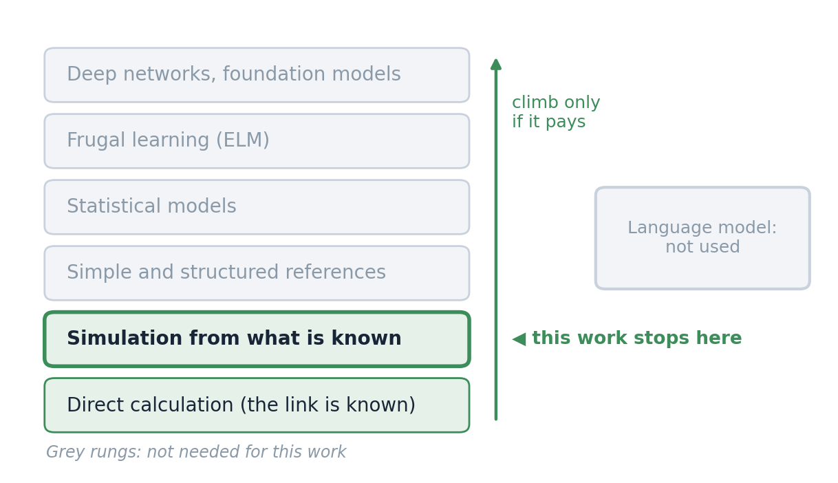
Model first. The link between the activity given and the response of the tumour is described by an explicit model, calibrated on patients; learning will be added only where it falls short (hybrid twin, in progress).
Definitions
- \(A(t)\)
- activity of the radioactive iodine present (GBq)
- \(N(t)\)
- number of tumour cells
- \(Tg(t)\)
- thyroglobulin in the blood (ng/mL), the clinical biomarker
- \(D,\ n,\ \Delta T\)
- activity per session (GBq), number of sessions, interval between sessions (months)
- \(T_d\)
- tumour doubling time (months): what separates a refractory from a responding profile
Equations
$$\frac{dA}{dt}=-a\ln2\,A,$$ $$\frac{dN}{dt}=N\left(\frac{\ln2}{T_d}-r_0\,A\right),$$ $$\frac{dTg}{dt}=\lambda\,N-k_e\,Tg .$$The activity decays at the effective rate \(a\ln2\) (radioactive and biological clearance together); the tumour grows at \(\ln2/T_d\) and is killed in proportion to cells and activity present; thyroglobulin is secreted by the tumour cells and cleared at rate \(k_e\).
Session by session
At session \(i\), a bolus \(D\) is added to the residual activity, \(A_i=D+A_{i-1}e^{-a\ln2\,\Delta T}\). Between sessions, with \(t\) counted from the session:
$$A(t)=A_i\,e^{-a\ln2\,t},$$ $$N(t)=N_i\exp\!\left(\frac{\ln2}{T_d}\,t-\frac{r_0A_i}{a\ln2}\left(1-e^{-a\ln2\,t}\right)\right),$$ $$Tg(t)=e^{-k_et}\left(Tg_i+\lambda\int_0^t N(s)\,e^{k_es}\,ds\right).$$The values at the end of an interval are the initial conditions of the next one; the original code solves each interval symbolically (MATLAB dsolve).
Reading the model: an activity threshold
The tumour shrinks while the kill term exceeds growth, that is while the activity present exceeds
$$A^{*}=\frac{\ln2}{r_0\,T_d},$$that is \(A^{*}\approx 2.6\) GBq for the responding profile (\(T_d=66.6\) months) and \(A^{*}\approx 17.4\) GBq for the refractory one (\(T_d=9.8\) months).
One session of 3.7 GBq is above the threshold of the responding profile, not of the refractory one; for the latter, only the activity accumulated over sessions (about 26 GBq after the eighth session every 3 months, in this model) crosses it. This is why the two profiles react so differently to the same protocol.
Parameters of the public demonstrators
| Symbol | Value | Unit | Meaning |
|---|---|---|---|
| \(a\) | 0.0169 | month⁻¹ | effective decay of the activity (rate \(a\ln2\)) |
| \(r_0\) | 0.00407 | GBq⁻¹ month⁻¹ | radiation-induced kill rate |
| \(\lambda\) | 3.86 × 10⁻⁹ | ng mL⁻¹ month⁻¹ per cell | thyroglobulin secretion |
| \(k_e\) | 0.319 | month⁻¹ | thyroglobulin clearance |
| \(N_0,\ Tg_0\) | 1.12 × 10⁹, 100 | cells, ng/mL | initial conditions |
| \(T_d\) | 9.8 / 66.6 | months | refractory / responding archetype |
Assumptions and validity
Parameters calibrated on a cohort of 50 patients (MCMC-SAEM, Monolix) and shared by the two archetypes except \(T_d\); a deliberately simple description of residual activity and tumour response. A research tool, not a clinical decision tool; prospective validation is needed.
Try it in your browser
Choose a profile and a protocol (sessions, interval, activity) and follow thyroglobulin over 80 months, with the activity threshold A*.
Run it
Python 3, NumPy and SciPy; executed on 23 October 2026. The values match the original MATLAB demonstrators to within 0.02 ng/mL (difference due to the sampling of fplot).
import numpy as np
from scipy.integrate import solve_ivp

# parameters of the public demonstrators (github.com/MarieFG49/CTD_SIMU_RAI)
r0, a, lam, ke = 0.00407, 0.0169, 3.86e-9, 0.319
N0, Tg0 = 1.12e9, 100.0
k = a * np.log(2)


def tg_at(t_end, Td, n_sessions, lag=3.0, dose=3.7):
    N, Tg, A_res, t0 = N0, Tg0, 0.0, 0.0
    for i in range(n_sessions):
        A0 = dose + A_res                     # new bolus on top of the residual activity
        t1 = (i + 1) * lag if i < n_sessions - 1 else t_end
        rhs = lambda t, y: [y[0] * (np.log(2) / Td - r0 * A0 * np.exp(-k * (t - t0))), lam * y[0] - ke * y[1]]
        N, Tg = solve_ivp(rhs, (t0, t1), [N, Tg], rtol=1e-10, atol=1e-6, method="LSODA").y[:, -1]
        A_res, t0 = A0 * np.exp(-k * lag), t1
    return Tg


for Td in (9.8, 66.6):
    print(f"Td = {Td:4} months: Tg(79) = {tg_at(79, Td, 1):8.2f} ng/mL after 1 session, {tg_at(79, Td, 8):6.2f} after 8")
Output:
Td =  9.8 months: Tg(79) =  1385.54 ng/mL after 1 session,  12.06 after 8
Td = 66.6 months: Tg(79) =    14.01 ng/mL after 1 session,   0.13 after 8
The original code (MATLAB, Symbolic Math Toolbox): main_demonstrateur98f and main_demonstrateur666f sweep the number of sessions, the interval and the activity for each archetype; SIMULATEUR1VF2024 opens the interactive simulator.
Results of the demonstrators
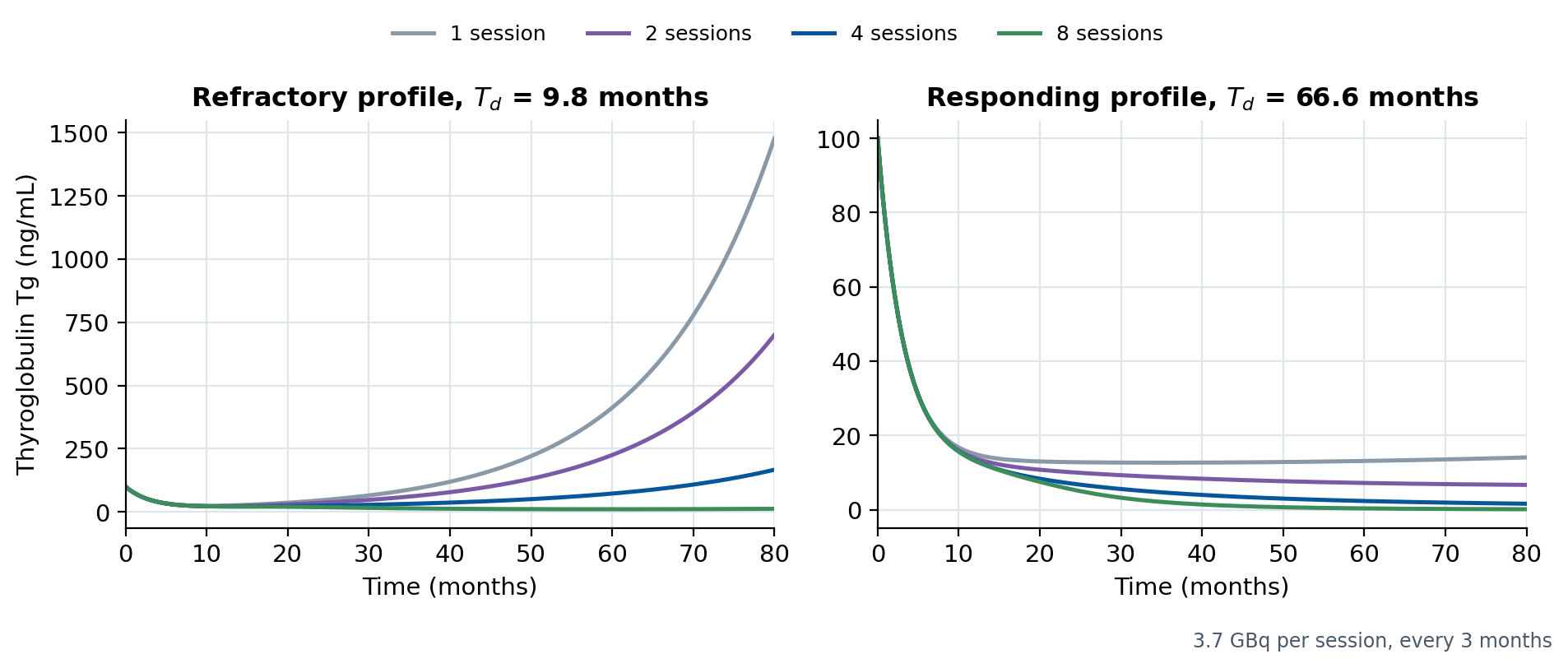
The public demonstrators share every parameter except the tumour doubling time: Td = 9.8 months for a refractory profile and 66.6 months for a responding one. With 3.7 GBq per session every 3 months:
| Profile | Td (months) | Tg at 79 months, 1 session (ng/mL) | Tg at 79 months, 8 sessions (ng/mL) |
|---|---|---|---|
| Refractory | 9.8 | 1,385.5 | 12.1 |
| Responding | 66.6 | 14.0 | 0.13 |
For the refractory profile, a single session only delays the regrowth: thyroglobulin climbs again after about a year. Eight sessions keep it low. For the responding profile, one session already brings thyroglobulin down; more sessions push it towards zero. These are model outputs for two archetypes, not predictions for a patient.
What the published study does
All parameters, including the doubling time itself, were calibrated on a cohort of 50 patients with the MCMC-SAEM algorithm (Monolix). The study then runs a sensitivity analysis of the three protocol parameters (number of sessions, interval between sessions and activity per session) on the thyroglobulin kinetics, and identifies the tumour doubling time as the quantity that separates responding from refractory profiles.
Towards a hybrid digital twin
The next step keeps the model at the core and adds learning only where it falls short: a hybrid digital twin, in which a frugal learner (an extreme learning machine, for example) estimates what the three equations do not capture, informed by medicine and mathematics rather than replacing them. This work is in progress and separate from the published results.
Limits
Two archetypes and population-calibrated parameters; residual activity and tumour response are described by a deliberately simple model. RAIR-Sim is a research tool: it is not a clinical decision tool and has not been validated prospectively.
Links
| Publications |
|
|---|---|
| Code | github.com/cyrilvoyant/CTD_SIMU_RAI |
| Archive (all versions) | doi:10.5281/zenodo.21496197 (Zenodo) |
| Software Heritage | permanent archive of the repository |
| Original code | RAIR-Sim by Marie Fusella Giuntini: github.com/MarieFG49/CTD_SIMU_RAI (MIT); the row above is the documented fork |
| For everyone (in French) | IA et cancer de la thyroïde : demain, la fin des traitements standardisés ? (in French), The Conversation, May 2026 |
| The story, for everyone | Thyroid cancer and radioiodine: model first · en français |
| The approach | Concentric modeling: understand before you compute |
| Author | Cyril Voyant (Mines Paris – PSL, O.I.E.) · ORCID · www.cyrilvoyant.com |
Related guides
LQL-Equiv: radiobiological dose equivalence · One ELM for seven grid signals · The approach: understand before you compute
Authors and source
M. Fusella Giuntini, C. Voyant, D. Taieb, D. Barbolosi, A computational framework for optimizing radioiodine therapy protocols in metastatic thyroid cancer, Scientific Reports 16, 27179 (2026), doi:10.1038/s41598-026-56267-1. The simulator RAIR-Sim was written by Marie Fusella Giuntini (github.com/MarieFG49/CTD_SIMU_RAI, MIT). Cyril Voyant wrote this page; the work belongs to the full author team.