Solar forecasting explained · 22 October 2026 · Published article, open code
How variable is the sun, and how forecastable? sCV and F explained
Before choosing a forecasting model, it helps to know how difficult the site is. Two numbers answer that: sCV, the variability that clouds add to the course of the sun, and F, how much of that variability can be anticipated at a given horizon.
Why the usual coefficient of variation misleads
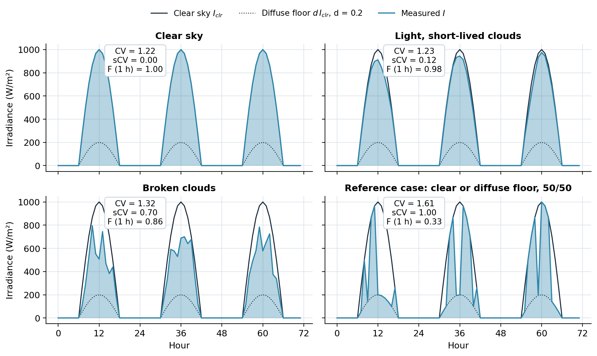
The coefficient of variation CV = σ/μ mostly measures the day: the sun rises and sets, so a perfectly clear sky already has a large CV (about 1.2 in the figure below). Two sites with the same clouds but different day lengths get different CVs. A forecaster needs the part the sun's course does not explain: the clouds.
sCV: variability around clear sky
sCV measures the spread of the measured irradiance I around the clear-sky irradiance Iclr, not around the mean:
sCV = √2 / |d − 1| × RMSE(I, I_clr) / √(σ_clr² + μ_clr²)- RMSE(I, Iclr) is the error of the clear-sky model used as a forecast;
- √(σclr² + μclr²) is the root mean square of the clear-sky curve;
- d = 0.2 is the diffuse floor: the fraction of clear sky that remains under a thick cloud.
sCV = 0 for a clear sky and 1 for the most variable sky the article considers, one that switches at random between clear sky and the diffuse floor. Night hours change nothing.
F: forecastability at a horizon
With ε = I − Iclr and ρmax the largest autocorrelation of ε over the lags from the horizon n to half a day:
F = 1 + sCV × (ρ_max − 1)F lies between 1 − sCV (clouds with no memory) and 1 (clouds that last). A cloudy site can be forecastable if its clouds persist; a site with fast, random clouds is not. sCV describes the site; F describes the forecasting task at a horizon.
Worked example by hand
| Hour | Clear sky | Measured | Difference |
|---|---|---|---|
| 1 | 400 | 400 | 0 |
| 2 | 800 | 500 | −300 |
| 3 | 800 | 760 | −40 |
| 4 | 400 | 200 | −200 |
- RMSE of clear sky: √(131 600 / 4) ≈ 181.4 W/m².
- Root mean square of clear sky: √(1 600 000 / 4) ≈ 632.5 W/m².
- sCV = √2 / 0.8 × 181.4 / 632.5 ≈ 0.51.
- If the residuals keep ρmax = 0.6 at the horizon of interest: F = 1 + 0.51 × (0.6 − 1) ≈ 0.80.
Fictitious teaching values.
F predicts forecast error
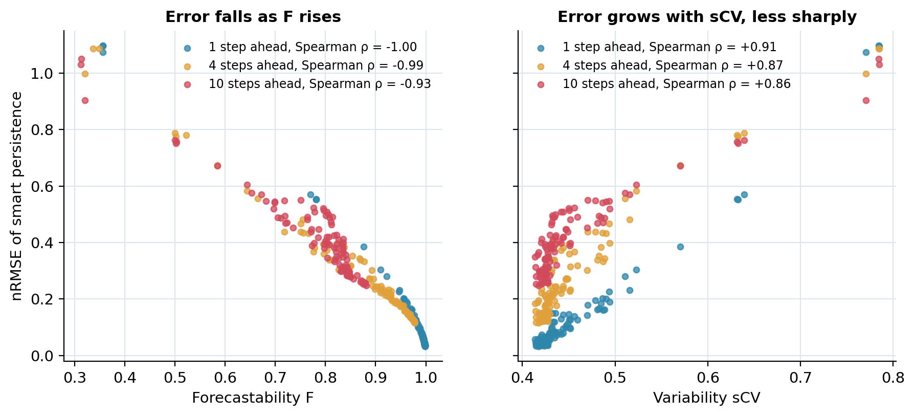
This is the article's conclusion on synthetic series and on 68 stations of the Spanish SIAR network: F is the better predictor of how hard forecasting will be, sCV the better description of variability. Use at least a year of data and a time step of a few minutes or more.
Code
The repository gives scv.m and forecastability.m (base MATLAB), a demonstration that writes the figures above, and the article's own scripts, unchanged.
s = scv(I, I_clr);                       % d = 0.2
F = forecastability(I, I_clr, 24, 1);    % hourly data, one hour ahead
MATLAB code and demonstrationRelated: NICE metrics
Authors and source
Article: Cyril Voyant, Alan Julien, Milan Despotovic, Gilles Notton, Luis Antonio Garcia-Gutierrez, Claudio Francesco Nicolosi, Philippe Blanc, Jamie Bright. Stochastic coefficient of variation: Assessing the variability and forecastability of solar irradiance. Renewable Energy 256 (2026) 123913. Cyril Voyant wrote this page; the method belongs to the full author team.